Why? Link to heading

After following Andrej Karpathy’s tutorial micrograd and the c231 notes (probably written by Andrej as well). Santiago and I decided that it was a good idea that in order to deepen our understanding of Convolutional Neural Networks (CNN) and appreciate the efficiency of PyTorch, we would be implementing a simple CNN from scratch with the micrograd code that we had.

In this post, we explain what we did and publish our notebook here. It’s a simple CNN model with the standard MNIST dataset. I would say the second most interesting thing I’ve learned going through this project, beside the autograd implementation, is learning how the parameters are initialized in a PyTorch NN model.

Commons Link to heading

Dataset Link to heading

We utilize CIFAR10 dataset.

Model architecture Link to heading

Level 1: Standard implementation with `torch.nn.module` Link to heading

We start with a simple CNN architecture which is implemented with torch.nn.module as follows. With 1 convolutional layer (in_channel = 1, out_channel 2), 1 max-pool layer (4x4) and 1 fully connected layer for final classification. We are aware that this is not good enough for MNIST, but this choice is for the purpose of computation efficiency. We are trying to demonstrate that the autograd we’ve built runs correctly in the CNN architecture.

class SimpleCNN(nn.Module):
    def __init__(self):
        super(SimpleCNN, self).__init__()
        
        self.conv1 = nn.Conv2d(1, 2, kernel_size=3, padding=1)
        self.pool = nn.MaxPool2d(4, 4)
        self.fc1 = nn.Linear(2 * 7 * 7, 10) 

    def forward(self, x):
        x = self.pool(F.relu(self.conv1(x)))       
        x = x.view(x.size(0), -1)                  
        x = self.fc1(x)
        return x

Also, we are running with only a batch of 3 images. This is an example of how we retrieve such a batch.

transform = transforms.Compose([
    transforms.ToTensor(),
    transforms.Normalize((0.1307,), (0.3081,))
])

trainset = torchvision.datasets.MNIST(root='/tmp/data', train=True, download=True, transform=transform)

images = torch.stack([trainset[i][0] for i in range(3)])
labels = torch.stack([trainset[i][1] for i in range(3)])

Let us re-hash the basic of training a model: Link to heading

Initialization of model and it’s optimizer (here we are setting the learning rate as 0.01).
Put the batch of images through the model, which produces output logits used for prediction.
With the output prediction, we calculate the training loss (here we’re using mean square error with one-hot encoded labels).
Reset the gradients of the NN’s parameters.
Back-propagate from the batch’s loss value to calculate the gradients of the parameters.
Update the paramters’ values based on the the gradients and learning rate, via the optimizer.

The sample code of this process is as bellow:

model = SimpleCNN()
opt = torch.optim.SGD(model.parameters(), lr = 0.01)
output = model(images)
labels_one_hot = F.one_hot(labels, num_classes=10).float()
labels_one_hot.requires_grad_(False)
loss = F.mse_loss(output, labels_one_hot)
opt.zero_grad()
loss.backward()
opt.step()

Some more basics of an `nn.Module` model before we move on Link to heading

You can actually see the model’s parameters via the following script
```
for n, p in model.named_parameters():
    print(n, p.data)
```
The result (ommitted) will take the following form:
```
conv.weight tensor( ... )
conv.bias tensor( ... )
fc.weight tensor( ... )
fc.bias tensor( ... )
```
Note this form that the parameters, which corresponds with the layers we initialized. In the next level, we are going to try and replicate this which are automated by torch’s nn.Module.
You can see the gradients of the parameters after you’ve perform the back-propagation operation with the following script
```
for n, p in model.named_parameters():
    print(n, p.grad)
```
The result format is similar to the parameters’ printout.
The optimizer is basically a predefined algorithm which update the parameters based on the gradients and learning rate according to the following formula (we purposefully select the simplest one): $$ \theta = \theta - \eta \nabla_\theta J(\theta) $$

where:
- $\theta$: the model parameters (e.g., weights and biases)
- $\eta$: the learning rate (controls the step size)
- $J(\theta)$: the loss function with respect to $\theta$
- $\nabla_\theta J(\theta)$: the gradient (vector of partial derivatives) of the loss function with respect to $\theta$

Level 2: Breaking it down using `torch.nn.functional` Link to heading

Detour: Copying the parameter initialization mechanism Link to heading

Low-Level Implementation Link to heading

For maximum control and understanding, we can implement CNN operations from scratch using basic tensor operations.

def conv2d_manual(inputs, kernel):
    # Manual implementation of 2D convolution
    batch_size, height, width, channels = inputs.shape
    kernel_size = kernel.shape[0]
    output = np.zeros((batch_size, height, width, kernel.shape[-1]))
    
    for b in range(batch_size):
        for h in range(height):
            for w in range(width):
                for k in range(kernel.shape[-1]):
                    for i in range(kernel_size):
                        for j in range(kernel_size):
                            if h+i < height and w+j < width:
                                output[b,h,w,k] += np.sum(
                                    inputs[b,h+i,w+j,:] * kernel[i,j,:,k]
                                )
    return output

When to Use Each Level? Link to heading

High-Level: Best for rapid prototyping and production applications
Mid-Level: Useful when you need custom layers or specific optimizations
Low-Level: Ideal for learning and understanding the underlying mathematics

Conclusion Link to heading

Understanding these different implementation levels helps you choose the right approach for your specific needs. Whether you’re building a production system or learning the fundamentals, there’s an appropriate level of abstraction for your use case.

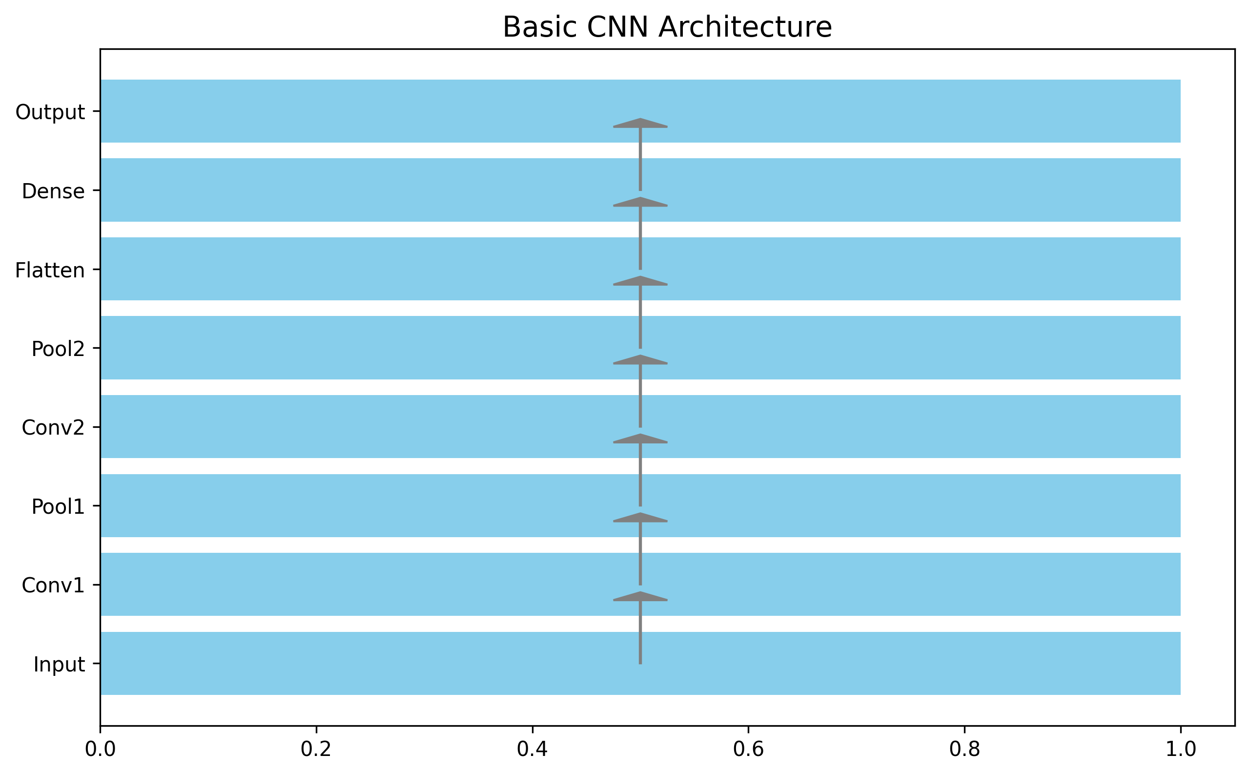Figure 1: Basic CNN Architecture

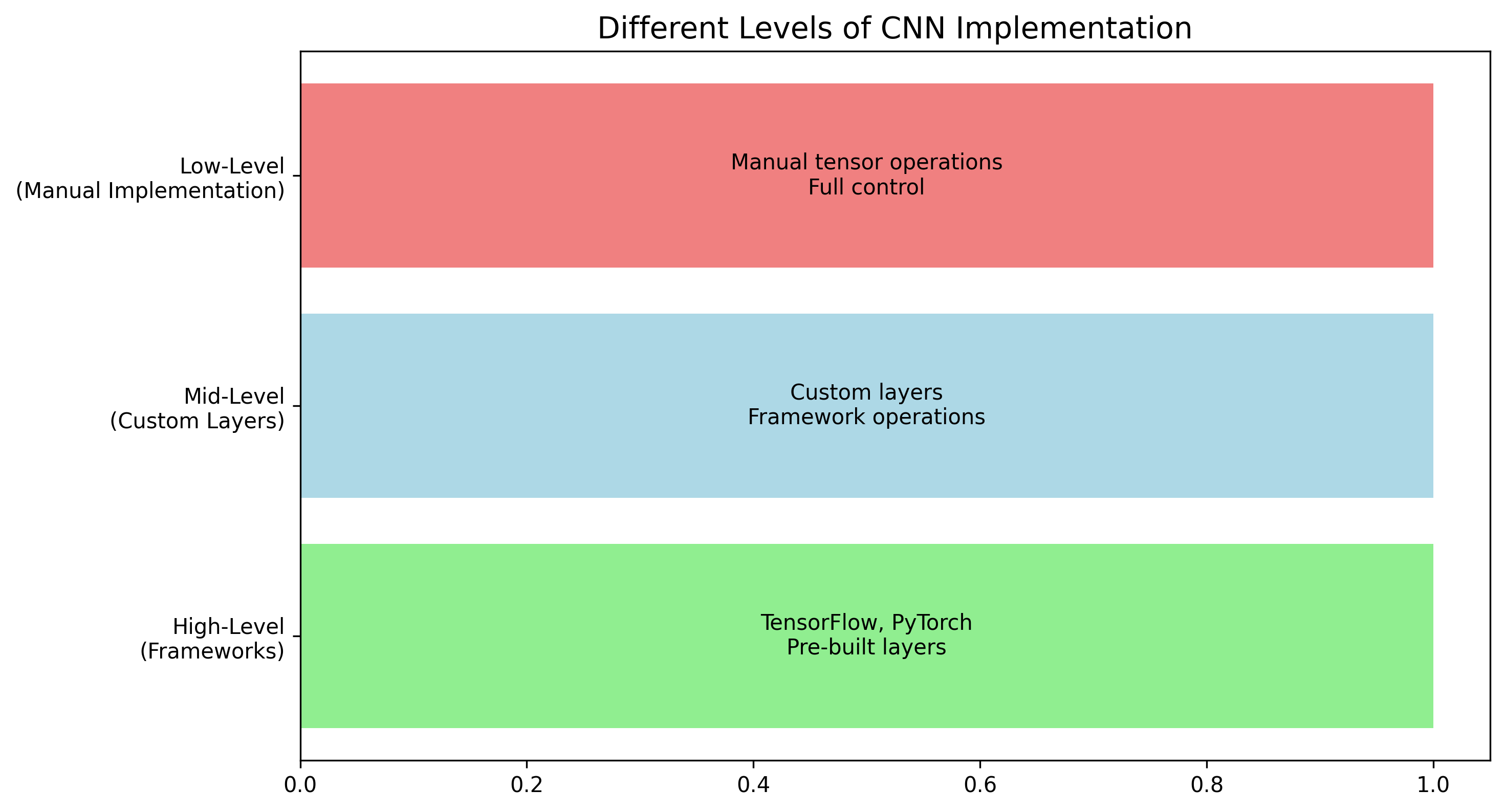Implementation Levels Figure 2: Different Levels of CNN Implementation